Colorization using Optimization

Anat Levin이 2004년 SIGGRAPH에 발표한 논문으로, colorization 과정에 optimization을 도입한 최초의 논문이다.

24년 수강했던 오태현 교수님의 영상처리 (Image Processing) 수업에서 다루었던 논문으로, 해당 논문을 주제로 기말 프로젝트를 수행하며 깊게 공부하였다.

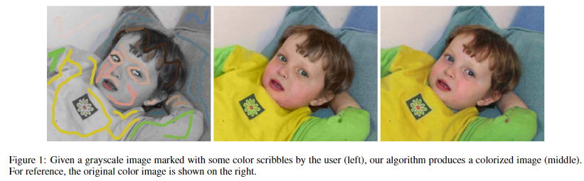
한줄 요약하자면 사람이 직접 색상 힌트를 조금만 줘도 그 힌트를 constraint로 사용하여 최적화 과정을 거쳐 채색을 완료하는 알고리즘이다.

Abstract

Colorization은 monochrome 이미지를 컴퓨터의 도움을 받아 채색하는 과정이다. 그러나 채색을 위한 사람의 조작은 굉장히 지루하고, 시간이 많이 들고, 비싼 task이다.

이 논문에서는 간단한 colorization method를 제안한다. (정확한 영상 분할이나 지역 추적 없이!)

💡 Simple premise: neighboring pixels in space-time that have similar intensities should have similar colors

구체적으로는, using a quadratic cost function & obtain an optimization problem - 기존 테크닉들로 풀 수 있다!

아티스트들은 약간의 색상 scribbles만으로도 그것이 공간/시간적으로 propagated되어 채색이 완료된다.

1. Introduction

A major difficulty with colorization→it is an expensive and time-consuming process.

불행히도, automatic segmentation 알고리즘은 복잡한 경계를 식별하는 데 실패하곤 한다. (머리카락 등!)

이 논문은 새로운 interactive colorization 기술을 고안한다. 수동 분할(segmentation)도 필요 없고 accurate tracking도 필요 없다. 이 기술은 정지 영상과 영상 시퀀스 모두에 적용 가능한 통합 프레임워크를 기반으로 한다. User는 정확한 경계선 추적 대신 각 구역의 색깔 정보만 scribbles 남기면 이것들을 constraints로 하여 자동적으로 인근 픽셀들로 색상 정보를 전파한다. 이 아이디어를 통해 영상에서 인근 프레임으로의 색상 전파도 가능하다.

Nearby pixels in space-time that have similar gray levels should also have similar colors.

2. Algorithm

YUV color space를 가정한다. (Y: monochromatic luminance, U, V: chrominance channels, encoding the color)

간단히 말하자면 Y는 밝기 정보, U는 Blue와 Y의 차이, V는 Red와 Y의 색차이다. 정확한 변환식은 아래와 같다. \(Y=(0.257\times R)+(0.504\times G)+(0.098\times B)+16\ U=-(0.148\times R)-(0.291\times G)+(0.439\times B)+128\ V=(0.439\times R)-(0.368\times G)-(0.071\times B)+128\) 선형 변환이기 때문에 YUV에서 RGB로의 역변환 역시 가능하다.

본 알고리즘의 입출력은 아래와 같다.

• Input: Intensity volume $Y(x,y,t)$
• Output: two color volumes $U(x,y,t), V(x,y,t)$

본 알고리즘에서 objective function (Cost function)은 아래와 같다. \(J(U)=\sum_r \left( U(\mathbf{r})-\sum_{\mathbf{s}\in N(\mathbf{r})}w_{\mathbf{rs}}U(\mathbf{s})\right) ^2\)

는 이웃한 두 픽셀의 $(x,y,t)$이고 $w_{\mathbf{rs}}$는 모두 합하면 1이 되는 weight function이다. (클수록 비슷한 것, 작을수록 두 점의 intensity가 다른 것)

우리는 두 이웃한 픽셀의 intensity가 비슷하면 색도 비슷하도록 하는 constraint를 도입하는 것이다. 이를 위해, 한 픽셀의 U와 이웃한 픽셀들의 U들의 weighted sum의 차를 최소화하도록 한다.

$w_{\mathbf{rs}}$는 본 논문에서 두 가지를 적용하여 실험해본다.

\[w_\mathbf{rs} \propto e^{Y(\mathbf{r})-(Y(\mathbf{s}))^2/2\sigma_\mathbf{r}^2}\ w_\mathbf{rs} \propto1+\frac{1}{\sigma_\mathbf{r}^2}(Y(\mathbf{r})-\mu_\mathbf{r})(Y(\mathbf{s})-\mu_\mathbf{r})\]

• $\mu_\mathbf{r} , \sigma_\mathbf{r}$ 은 $\mathbf{r}$ 주위 window의 평균과 분산이다.
• 첫 번째는 squared difference, 두 번째는 두 intensities 사이의 normalized correlation이다.

U는 linear function of intensity Y이다.

즉, $U=a_iY+b_i$이며 neighbor 픽셀들끼리는 a와 b가 같다.

intensity가 constant → color should be constant

intensity가 edge → color should be edge

이 모델은 시스템에 각 이미지 윈도우마다 pair of variables를 추가하지만, 간단하게 a, b variables를 제거함으로써 correlation-based affinity function 식을 얻을 수 있다.

Neighbor 정의

$N(\mathbf{r})$은 $\mathbf{r}$의 neighbor라는 뜻.

Single Frame: locations are nearby → neighbors

b/w two successive frames: if their image locations after accounting for motion are nearby →neighbors

조금 더 구체적으로는, $\nu_x(x,y), \nu_y(x,y)$가 time $t$에서 계산된 optical flow일 때, 두 픽셀 $(x_0,y_0,t), (x_1,y_1,t)$는 아래 수식이 성립할 때 neighbor이다. \(||(x_0+\nu_x(x_0),y_0+\nu_y(y_0))-(x_1,y_1)||<T\)

이 때 optimal flow $\nu$를 계산하는 것은 1981년 논문 Lucas and Kanade’s standard motion estimation algorithm.의 것을 따른다.

이 때 optical flow는 두 픽셀의 이웃 여부에서만 사용되고 propagation에서는 사용되지 않는다.

After the user’s scribbles

• $\mathbf r_i$: a set of locations where the colors are specified by user’s scribbles
• $u(\mathbf{r}_i)=u_i, v(\mathbf{r}_i)=v_i$: 유저가 제시해준 픽셀 $\mathbf{r}$의 색깔 (YUV에서 U,V)

우리는 위의 constraints를 활용하여 $J(U),J(V)$를 minimize해야 한다.

objective function이 quadratic(2차)이고 constraints가 linear하기 때문에 이 optimization problem에서 large, sparse system of linear equations를 얻을 수 있다. (몇몇 standard methods로 풀 수 있다)

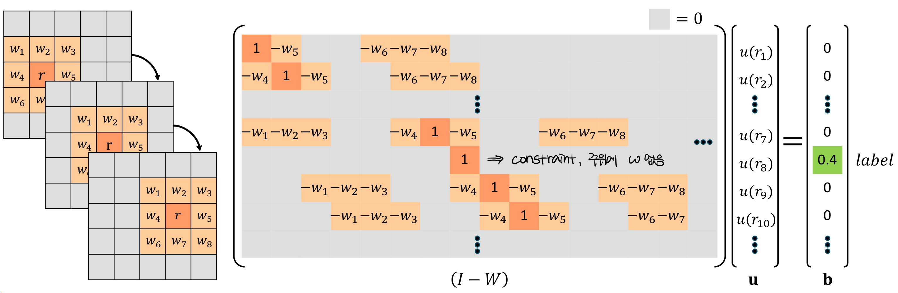
Sparse Linear System (in EECE490G Lec.5)

Objective function $J(U)=\sum_r \left( U(\mathbf{r})-\sum_{\mathbf{s}\in N(\mathbf{r})}w_{\mathbf{rs}}U(\mathbf{s})\right) ^2$

Matrix form of above $ J(U)=\Vert(I-W)\mathbf{u}\Vert^2 $, same as find $ \text{argmin}\lim _{U} {\left\Vert(I-W)\mathbf{u}\right\Vert^2} $

constraint

\[(I-W)\mathbf{u}=\mathbf{b}, \quad b(\mathbf{r}_i)= \begin{cases} 0, & \mathbf{r}_i \text{ w/o label} \\ u(\mathbf{r}_i), & \mathbf{r}_i \text{ w/ label} \end{cases}\]

• $I,W\in \mathbb{R}^{HW\times HW} \ \mathbf{u,b}\in \mathbb{R}^{HW}$